People from statistical background can quickly understand Cohort Table or Analysis, but I don’t remember learning it during my undergraduate and postgraduate studies or as a choice I ought to have skipped it, ha ha! When I did google and explored few basic examples, it did not take long for me to understand cohort table/analysis. It is however harder for me to build the same cohort table in Adobe Analytics Workspace because of the multiple components available to construct the cohort. I know that experts have no trouble in understanding the components but not for all and thus the post.
The following components are required to build a cohort table in Adobe Analytics. Few are mandate while the rest are optional or add capabilities to the table of cohort.
- Metric
- Inclusion Criteria
- Return Criteria
- Granularity
- Type
- Settings
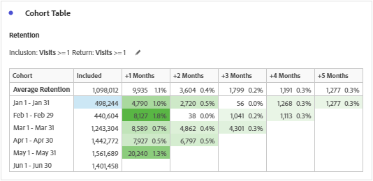
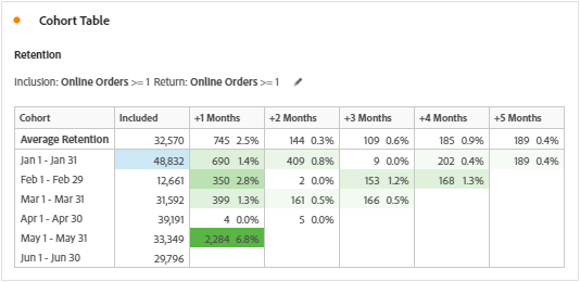
A cohort is a group of visitors who share a common characteristic over a certain period of time. There are multiple use cases for cohort analysis and is available in the link here. As previously said, we would concentrate on the table components instead of cohort use cases. So let’s take the use case Website Visitor Retention based on Visits and Orders during the months between January 2020 and June 2020 to understand the components. Note that only dummy numbers are used for the analysis and are not absolute.
Metric
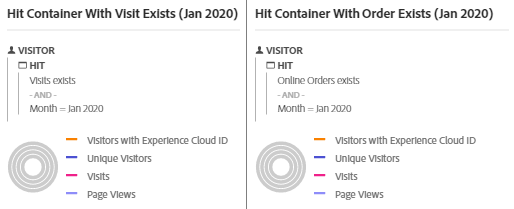
Unique Visitor is the only available and measurable metric in the cohort table. It is believed that the metrics are available according to the inclusion and return criteria, but is not correct. Metrics selected during inclusion or return criteria are segmented to Unique Visitor in correlation with the time period and the inclusion or return events. Note that the correlations are based on the Hit containers nested inside a Unique Visitor container. Below are the segments created based on the time period (To give you an idea, I used January 2020) when we add the metrics Visits and Orders to cohort table.

Inclusion Criteria
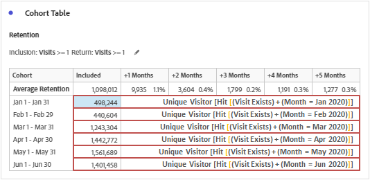
Inclusion criteria represents the column ‘included’ in the table of cohort. This is computed in the same way as we discussed above depending on the selected metrics and the time period.
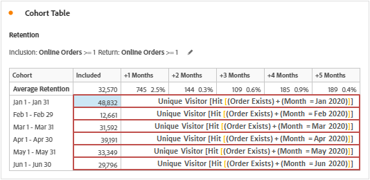
Additional notes:
– Metrics can also be constricted based on conditions and a maximum of 3 metrics can be added based on ‘AND’ or ‘OR’ logical operators.
– Maximum of 10 segments can be appended in addition to the metrics selected.
– Adding a metric & a segment or adding multiple segments will results in the logical operation ‘AND’.
Return Criteria
Return criteria represent the rest of columns (Months) in the table of cohort. Although the columns except ‘included’ depends on return criteria, the computation is based on both inclusion and return events. Let’s see how cell values are determined in row 1 for easier understanding.
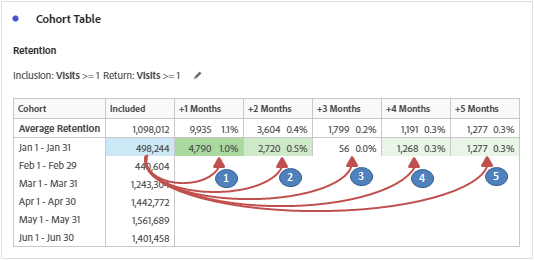
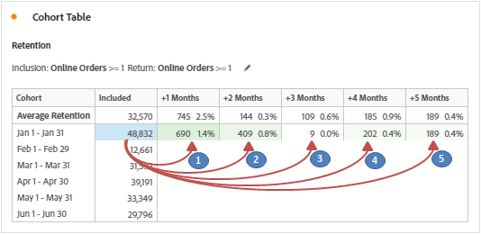
1. Inclusion Criteria for Jan 2020 + Return Criteria for Feb 2020 (+1 Month) i.e. Nested Unique Visitor containers based on the metric/segment selection and the time period. Have given the nested containers for both the tables of cohort for easier understanding.
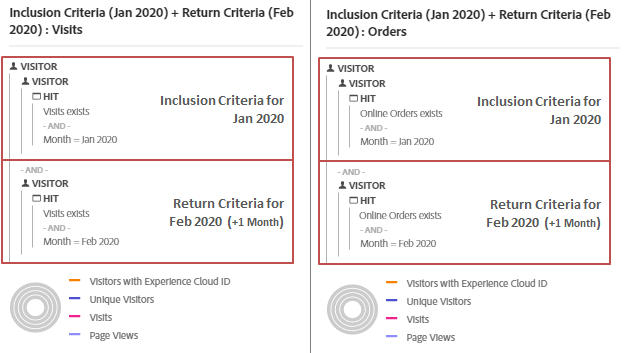

We can see that the segment results are matching the ‘+1 Months’ cell values of row 1 (Both Visits & Orders). Same applies to other column values of row 1, only the month on return criteria is to be modified i.e. March (+2 Month), April (+3 Month), May (+4 Month) etc. So, below are the additional segments for row 1.

For every row, the computation is the same but with different time period for the inclusion criteria (Feb 2020, Mar 2020, Apr 2020 etc.) and return criteria (+1 month, +2 month, +3 month etc.).
Additional notes:
– Metrics can also be constricted based on conditions and a maximum of 3 metrics can be added based on ‘AND’ or ‘OR’ logical operators.
– Maximum of 10 segments can be appended in addition to the metrics selected.
– Adding a metric & a segment or adding multiple segments will results in the logical operation ‘AND’.
– Percentage calculation is based on cell values of return criteria divided by inclusion criteria. i.e. 4,790 / 498,244 = 1.0% for Visitor Retention (Visits) and 690 / 48,832 = 1.4% for Visitor Retention (Orders).
Granularity
The time granularity of Day, Week, Month, Quarter, or Year. Important note is that we can only have maximum of 15 rows in the table of cohort i.e. 14 columns.
Type
Retention: Whatever we have discussed above is the type retention (Default). It is indicated by the color green in the table.
Churn: Churn is just the opposite of retention i.e. Churn = 1 – Retention. To obtain the cell values of churn, simply subtract the retention cell values of return criteria with the corresponding row values of inclusion criteria. Note that row values of inclusion criteria are same for both retention & churn and it is indicated by the color red in the table.
Settings
Rolling Calculation
The cell values computation of return criteria change when we apply rolling calculation to the cohort table. In default computation, the return criterion month changes based on the columns, however in rolling calculation, the months are appended.
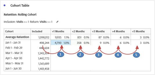
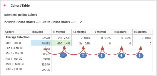
Said that, below is how the segment computation change for the cell values in row 1.


We can see that the segment results are matching the computation logic for the rolling calculation (Computed for ‘+1 Months’ & ‘+2 Months’ to give you an idea) and the computation is applicable to all other cell values of return criteria.
Latency Table
In latency table, the return criteria is applied to both before and after the inclusion event is occurred.

Since because the return criteria is applied to both before and after the inclusion event, below are how the segments will look like for row 1 of the cohort table (Visits & Orders) without rolling calculation.

And with rolling calculation, below are how the segments will look like.

The computation logic is similar for all other rows and columns i.e. Cell values.
Custom Dimension Cohort
Rather than the time based cohort, the computation is now based on the dimension or dimensional values selected. Rolling or default, the cell values are computed exactly the way we discussed above. Important is that we can have only the first line item of the time period (Here, Jan 2020) in the ‘included’ column since the time period values are replaced by the dimensional values i.e. Time period selection is tricky. On the other hand, cohort will return the top 14 dimension items but we can use a filter (access it by hovering on the right of the dimension that was dragged on) to display only the desired. And, a custom dimension cohort cannot be used with the latency table feature.
Other granular details such as average retention, round percentage, show percent etc., are just pedestals and didn’t require any delineation. Happy New Year 2021!


